Unit 3: Understanding Process Management of Operating System

UNIT 3 Process Management

Process

A process is defined as an entity which represents the basic unit of work to be implemented in the system i.e. a process is a program in execution. The execution of a process must progress in a sequential fashion. In general, a process will need certain resources such as the CPU time, memory, files, I/O devices and etc. to accomplish its task. As a process executes, it changes state. The state of a process is defined by its current activity. Each process may be in one of the following states: New state, ready state, waiting state, running state, and finished (Exit) state.

Process states

1.   New: A process that has just been created but has not yet been admitted to the pool of executable processes by the OS.

2.   Ready: Process that is prepared to execute when given the opportunity. That is, they are not waiting on anything except the CPU availability.

3.   Running: the process that is currently being executed.

4.   Blocked: A process that cannot execute until some event occurs, such as the completion of an I/O operation.

5.   Exit: a process that has been released from the pool of executable processes by the OS, either because it halted or because it aborted for some reason. A process that has been released by OS either after normal termination or after abnormal termination (error).

Fig: 5 state process model

Process state transition

1.   The New state corresponds to a process that has just been defined or newly born process. For example, if a new user attempts to log on to a time sharing system or if a new batch job is submitted for execution.

2.   New to Ready: process has been loaded into main memory and is pending execution on a CPU. There may be many "ready" processes at any one point of the system's execution—for example, in a one-processor system, only one process can be executing at any one time, and all other "concurrently executing" processes will be waiting for execution.

3.   Ready to Running: The OS selects one of the processes in the ready state for execution.

4.   Running to Exit: The currently running process is terminated by the OS if the process indicates that it is completed or if it aborts i.e. the process is terminated when it reaches a natural completion point. At this point process is no longer eligible for execution and all of the memory and resources associated with it are de-allocated so they can be used by other processes.

5.   Running to Waiting: A process may be blocked due to various reasons such as when a particular process has tired the CPU time allocated to it or it is waiting for an event to occur. A process is put in blocked or waiting state if it requests something for which it must wait. For example, a process may request a service from the OS and the OS is not prepared to perform immediately. It can request a resource such as file or a shared section of virtual memory that is not immediately available.

6.   Waiting to Ready: A process in the blocked state is moved to the ready state when the event for which it has been waiting occurs.

The state of process from ready to running, running to waiting and waiting to ready will be continued till the process terminates. This process is shown in above figure.

The Process Control Block (PCB)

A process control block or PCB is a data structure (a table) that holds information about a process. Every process or program that runs needs a PCB. When a user requests to run a particular program, the operating system constructs a process control block for that program. It is also known as Task Control Block (TCB). It contains many pieces of information associated with a specific process i.e. it simply serves as the respiratory for any information that may vary from process to process. The process control block typically contains:

·         An ID number that identifies the process

·         Pointers to the locations in the program and its data where processing last occurred

·         Register contents

·         States of various flags and switches

·         Pointers to the upper and lower bounds of the memory required for the process

·         A list of files opened by the process

·         The priority of the process

·         The status of all I/O devices needed by the process

Process state

Process ID number

Program Counter

CPU registers

Memory limits

List of open files

………

Fig: Process Control Block

The information stored in the Process Control Block in given below

·      Process ID: given by the CPU when the process request for the service.

·      Process State: The state may be new, ready, running, and waiting, halted, and so on.

·      Program Counter: the counter indicates the address of the next instruction to be executed for this process.

·      CPU register: The registers vary in number and type, depending on the computer architecture. They include accumulator, index registers, stack pointers, and general purpose registers. Along with the program counter, this state information must be saved when an interrupt occurs, to allow the process to be continued correctly afterward.

·      CPU Scheduling information: This information includes a process priority, pointers to scheduling queues, and other scheduling parameters.

·      Memory management information: this information include the value of the base and limit registers, the page table, or the segment tables, depending on the memory system used by the OS.

·      Accounting information: This information includes the amount of CPU and real time used, time limits, account numbers, job or process numbers and so on.

·      I/O status information: This information includes the list of I/O devices allocated to the process, a list of open files and so on.

Role of PCB:

The PCB is most important and central data structure in an OS. Each PCB contains all the information about a process that is needed by the OS. The blocks are read and/or modified by virtually every module in the OS, including those involved with scheduling, resource allocation, interrupt processing and performance monitoring and analysis that mean PCB defines the state of OS.

The PCB contains the information about the process. It is the central store of information that allows the operating system to locate all the key information about a process. When CPU switches from one process to another, the operating system uses the Process Control Block (PCB) to save the state of process and uses this information when control returns back process is terminated, the Process Control Block (PCB) released from the memory.

A context switch is the computing process of storing and restoring the state (context) of a CPU such that multiple processes can share a single CPU resource. The context switch is an essential feature of a multitasking operating system. Context switches are usually computationally intensive and much of the design of operating systems is to optimize the use of context switches. There are three scenarios where a context switch needs to occur: multitasking, interrupt handling, user and kernel mode switching. In a context switch, the state of the first process must be saved somehow, so that, when the scheduler gets back to the execution of the first process, it can restore this state and continue. The state of the process includes all the registers that the process may be using, especially the program counter, plus any other operating system specific data that may be necessary. Often, all the data that is necessary for state is stored in one data structure, called a process control block.

Fig: Showing CPU switches from process to process (Role of PCB)

Operations on processes (creation, Termination, Hierarchies, Implementation)

Process creation:

·         Processes may create other processes through appropriate system calls. The process which creates other process is termed as parent process and the created process is termed as its child.

·         Each process is given an integer identifier, termed its process identifier, or PID. The parent PID ( PPID ) is also stored for each process.

·         There are two options for the parent process after creating the child:

ü  Wait for the child process to terminate before proceeding. The parent makes a system call (Wait), for either a specific child or for any child, which causes the parent process to block until the wait( ) returns.

ü  Run concurrently with the child, continuing to process without waiting.

Process termination:

A process may call a system call (exit) to terminate itself or it may also be terminated by the system for a variety of reasons, some of them are:

·         The inability of the system to deliver necessary system resources.

·         In response to a KILL command or other un-handled process interrupts.

·         A parent may kill its children if the task assigned to them is no longer needed.

·         If the parent exits, the system may or may not allow the child to continue without a parent.

When a process terminates, all of its system resources are freed up, open files flushed and closed, etc. The process termination stat

Process hierarchy:

The Process Model

Cooperating Processes (Inter-process Communication, IPC)

Processes executing concurrently (parallel) in the OS may be either independent process or cooperating process. A process is independent if it cannot or be affected by other processes executing in the system. Any process that does not share data with any other process is independent. A process is cooperating if it can affect or be affected by other processes executing in the system. Any process that shares data with other process is a cooperating process.

Advantages of process cooperation:

·         Information sharing- such as shared files.

·         Computation speed-up – to run a task faster, we must break it into subtasks, each of which will be executing in parallel. This speed up can be achieved only if the computer has multiple processing elements (such as CPUs or I/O channels).

·         Modularity – construct a system in a modular function (i.e., dividing the system functions into separate processes).

·         Convenience – one user may have many tasks to work on at one time. For example, a user may be editing, printing, and compiling in parallel.

Inter-Process Communication (IPC) is a set of techniques for the exchange and synchronization of data among two or more threads in one or more processes. Interprocess communication is useful for creating cooperating processes. Processes may be running on one or more computers connected by a network. IPC techniques are divided into methods for message passing, synchronization, shared memory, and remote procedure calls (RPC). The method of IPC used may vary based on the bandwidth and latency of communication between the threads, and the type of data being communicated.

The common Linux shells all allow redirection. For example

$ ls | pr | lpr

It pipes the output from the ls command listing the directory's files into the standard input of the pr command which paginates them. Finally the standard output from the pr command is piped into the standard input of the lpr command which prints the results on the default printer. Pipes then are unidirectional byte streams which connect the standard output from one process into the standard input of another process. Neither process is aware of this redirection and behaves just as it would normally. It is the shell which sets up these temporary pipes between the processes.

There are two fundamental mechanisms for Interprocess communication.

Message Passing

In the message passing model, communication takes place by means of messages exchanged between the cooperating processes that mean it provides mechanism to allow processes to communicate and to synchronize their actions without sharing the same address space. It is particularly useful in distributed environment, where communicating processes may reside on different computers connected by a network. For example, a chat program used on World Wide Web could be designed so that chat participants communicate with one other by exchanging messages.

A message passing facility provides at least two operations: send (message) and receive (message). Messages send by a process can be of either fixed size or variable size. If process A and B wants to communicate, they must send messages to and receive messages from each other and a communication link must exist between them. The sender typically uses send () system call to send messages, and the receiver uses receive () system call to receive messages. The communication link can be established in varieties of ways and some methods for logically implementing a link and the send () / receive operations are:

·         Direct or indirect communication

·         Synchronous or asynchronous communication

·         Automatic or explicit buffering.

Shared Memory

Interprocess communication using shared memory requires communicating processes to establish a region of shared memory. Shared memory is a memory that may be simultaneously accessed by multiple programs with intent to provide communication among them. Typically, a shared memory region resides in the address space of the process creating the shared memory segment. Other processes that wish to communicate using shared memory segment must attach it to their address space. Now they can exchange information by reading and writing data in the shared areas. Since both processes can access the shared memory area like regular working memory, this is a very fast way of communication. On the other hand, it is less powerful, as for example the communicating processes must be running on the same machine, and care must be taken to avoid issues if processes sharing memory are running on separate CPUs and the underlying architecture is not cache coherent. Since shared memory is inherently non-blocking, it can’t be used to achieve synchronization.

It allows maximum speed and convenience of communication. It is faster than message passing, because the message passing system are typically implemented using system calls and thus requires the more time consuming task of kernel intervention but in shared memory systems, system calls are only required only to establish shared memory regions. Once shared memory is established, all accesses are treated as routine memory accesses, and assistance of kernel is not required.

Fig: Communication model (a) Message passing (b) Shared memory

Threads

Definitions of Threads

A thread is a separate part of a process i.e. a thread is the smallest unit of processing that can be performed in an OS. A process can consist of several threads, each of which execute separately. It is a flow of control within a process. It is also known as light weight process. For example, one thread could handle screen refresh and drawing, another thread printing, another thread the mouse and keyboard. This gives good response times for complex programs. Windows NT is an example of an operating system which supports multi-threading.

A thread is a basic unit of CPU utilization; it comprises a thread ID, a program counter, a register set, and a stack. It shares with other threads belonging to same process its code section, data section, and other operating resources, such as open files and signals. A traditional (or heavy weight) process has a single thread of control. If a process has multiple threads of control, it can perform more than one task at a time.

Fig: (a) Three processes with one thread each (b) A process with 3 threads

Thread Usage

Threads were invented to allow parallelism to be combined with sequential execution and blocking system calls. Some examples of situations where we might use threads:

·         Doing lengthy processing: When a windows application is calculating it cannot process any more messages. As a result, the display cannot be updated.

·         Doing background processing: Some tasks may not be time critical, but need to execute continuously.

• Concurrent execution on multiprocessors
• Manage I/O more efficiently: some threads wait for I/O while others compute
• It is mostly used in large server applications

User Space and Kernel Space Threads

·         User level threads are threads that are visible to the programmer and unknown to the kernel. Such threads are supported above the kernel and managed without kernel support.

·         The operating system directly supports and manages kernel level threads. In general, user level threads are faster to create and manage than are kernel threads, as no intervention from the kernel is required. Windows XP, Linux, Mac OS X supports kernel threads.

Difference between User Level & Kernel Level Thread

S. N.	User Level Threads	Kernel Level Thread
1	User level threads are faster to create and manage.	Kernel level threads are slower to create and manage.
2	Implementation is by a thread library at the user level.	Operating system supports creation of Kernel threads.
3	User level thread is generic and can run on any operating system.	Kernel level thread is specific to the operating system.
4	Multi-threaded application cannot take advantage of multiprocessing.	Kernel routines themselves can be multithreaded.

Benefits of Multithread

·         Resource sharing

Process can only share resources using shared memory or message passing method. Such techniques are explicitly arranged by the programmer. However, threads share the memory and resources of the process to which they are belong by default. It (Sharing of code and data) allows an application to have several different threads of activity within the same address space.

·         Responsiveness

It may allow a program to continue running even if part of it is blocked or is performing lengthy operations, which increases the responsiveness to the user.

·         Economy

Allocation of memory and resources for process creation is costly. Because threads share the resources of the process to which they belong, it is more economical to create and context-switch threads. It is much more time consuming to create and manage processes than threads.

·         Scalability

In multiprocessor architecture threads may run in parallel on different processors. A single threaded process can only run on one processor. Multithreading on a multi-CPU machine increases parallelism.

Multithreading Models (Many-to-one model, One-to-One Model, Many-to many model)

Multithreading is the ability of a program or an operating system process to manage its use by more than one user at a time and to even manage multiple requests by the same user without having to have multiple copies of the programming running in the computer

A multithread process contains several different flow of control within the same address space.  When multiple threads are running concurrently then this is known as multithreading, which is similar to multitasking. Multithreading allows sub-processes to run concurrently.

Basically, an operating system with multitasking capabilities will allow programs (or processes) to run seemingly at the same time. On the other hand, a single program with multithreading capabilities will allow individual sub-processes (or threads) to run seemingly at the same time.

One example of multithreading is when we are downloading a video while playing it at the same time. Multithreading is also used extensively in computer-generated animations.

A relationship must exist between user threads and kernel threads. There are three models related to user and kernel threads and they are:

·         Many- to- one model: it maps many user threads to single kernel threads.

·         One - to one model: it mach each user thread to a corresponding thread

·         Many - to - many models: It maps many user threads to a smaller or equal number of kernel threads.

1.   Many to one model:

It maps many user threads to single kernel threads. Thread management is done by the thread library in user space, so it if efficient but the entire process will block if a thread makes a blocking system call. Because only one thread can access the kernel at a time, multiple threads are unable to run in parallel on multiprocessors.

Fig: Many-to-one model

2.   One to one model:

It mach each user thread to a corresponding kernel thread. It provides more concurrency than the many-to-one model by allowing another thread to run when a thread makes a blocking system call i.e. it also allows multiple threads to run in parallel on multiprocessor. The drawback is that creating a user thread requires creating the corresponding kernel thread and the overhead of creating the corresponding kernel thread can burden the performance of an application.

Fig: One-to-one model

3.   Many- to - many model:

It multiplexes many user-level threads to a smaller or equal number of kernel threads. The number of kernel threads may be specific to either a particular application or a particular machine. This model allows the developer to create as many user threads as the user wishes and the corresponding kernel threads can run in parallel on a multiprocessor. In such case true concurrency is not gained because the kernel can schedule only one thread at a time.

Fig: Many-to-many model

Difference between Process and Thread

S.N	Process	Thread
1	It is heavy weight	It is light weight, which takes lesser resources than a process
2	Process switching needs interaction with OS	Thread switching does not need interaction with OS
3	In multiple processing environments each process executes the same code but has its own memory and file resources.	All threads can share same set of open files, child processes.
4	If one process is blocked then no other process can execute until the first process is unblocked.	While one thread is blocked and waiting, second thread in the same task can run.
5	Multiple processes without using threads use more resources.	Multiple threaded processes use fewer resources.
6	In multiple processes each process operates independently of the others.	One thread can read, write or change another thread's data.

Process Scheduling

Technical Terms:

·         Ready queue:    The processes waiting to be assigned to a processor are put in a queue called ready queue.

·         Burst time:       The time for which a process holds the CPU is known as burst time.

·         Arrival time:     Arrival Time is the time at which a process arrives at the ready queue.

·         Turnaround time: The interval from the time of submission of a process to the time of completion is the turnaround time.

·         Waiting time:    Waiting time is the amount of time a process has been waiting in the ready queue.

·         Response Time: Time between submission of requests and first response to the request.

·         Throughput: number of processes completed per unit time.

·         Dispatch latency – It is the time it takes for the dispatcher to stop one process and start another running.

·         Context switch: A context switch is the computing process of storing and restoring the state (context) of a CPU so that execution can be resumed from the same point at a later time. This enables multiple processes to share a single CPU.

·         I/O bound process: - The process which spends more of its time doing I/O operations than it spends doing computations are called I/O bound process.

·         CPU bound process: - The process that generates I/O request infrequently and uses more time for performing computations is called CPU bound process.

Optimal scheduling algorithm will have minimum waiting time, minimum turnaround time and minimum number of context switches.

Basic Concept 

Scheduling is the process of controlling and prioritizing messages sent to a processor. The process scheduler is the component of the operating system that is responsible for deciding whether the currently running process should continue running and, if not, which process should run next

There are two main objectives of the process scheduling and they are:

·         To keep the CPU busy at all times and

·         To deliver "acceptable" response times for all programs, particularly for interactive ones.

There is a module called process scheduler which has to meet these objectives by implementing suitable policies for swapping processes in and out of the CPU.

CPU scheduling is done in the following four circumstances:

·         When a process switches from the running state to the waiting state

·         When a process switches from the running state to the ready state (For example, when an interrupt occurs)

·         When process switches from the waiting state to the ready state (For example, at completion of I/O)

·         When a process terminates.

Type of scheduling:

Scheduler are responsible for management of jobs, such as allocating resources needed for any specific job, partitioning of jobs schedule parallel executing of tasks, data management, event correlation, and etc.

The process scheduler is the component of the operating system that is responsible for deciding whether the currently running process should continue running and, if not, which process should run next.

Types of schedulers: A multi programmed system may include as many as three types of scheduler:

1.   The long-term (high-level) scheduler:

·         It admits new processes to the system. Long-term scheduling may be necessary because each process requires a portion of the available memory to contain its code and data.

·         It determines which programs are admitted to the system for processing. Thus, it controls the degree of multiprogramming.

·         It determines which programs are admitted to the system for execution and when, and which ones should be exited.

·         Once admitted job or program becomes a process and is added to the queue for the short term scheduler.

·         This scheduler dictates what processes are to run on a system, and the degree of concurrency to be supported at any one time.

·         A long-term scheduler is executed infrequently - only when a new job arrives. Thus, it can be fairly sophisticated.

·         Long term schedulers are generally found on batch systems, but are less common on timeshared systems or single user systems.

·         Long-term scheduling performs a gate-keeping function. It decides whether there's enough memory, or room, to allow new programs or jobs into the system.

·         When a job gets past the long-term scheduler, it's sent on to the medium-term scheduler.

2.   Medium-term (intermediate) scheduling

·         It determines when processes are to be suspended and resumed.

·         The mid-term scheduler temporarily removes processes from main memory and places them on secondary memory (such as a disk drive) or vice versa. This is commonly referred to as "swapping out" or "swapping in"

·         The mid-term scheduler may decide to swap out a process which has not been active for some time, or a process which has a low priority, or a process which is page faulting frequently, or a process which is taking up a large amount of memory in order to free up main memory for other processes, swapping the process back in later when more memory is available, or when the process has been unblocked and is no longer waiting for a resource.

·         It controls which processes are actually resident in memory, as opposed to being swapped out to disk.

·         A medium-term scheduler (if it exists) is executed more frequently. To minimize overhead, it cannot be too complex.

·         The medium-term scheduler makes the decision to send a job on or to sideline it until a more important process is finished. Later, when the computer is less busy or has less important jobs, the medium-term scheduler allows the suspended job to pass.

3.   Short term scheduler:

·         It determines which of the ready processes can have CPU resources, and for how long.  This affects the processes which are in running, reading and blocked state.

·         The short term scheduler determines the assignment of the CPU to ready processes i.e. it decides which of the ready, in-memory processes are to be executed (allocated a CPU) next following a clock interrupt, an IO interrupt, an operating system call or another form of signal

·         It is also known as dispatcher.

·         It makes scheduling decisions much more frequently than the long-term or mid-term schedulers

·         The short-term scheduler takes jobs from the "ready" line and gives them the green light to run. It decides which of them can have resources and for how long.

·         The short-term scheduler runs the highest-priority jobs first and must make on-the-spot decisions.

·         For example, when a running process is interrupted and may be changed, the short-term scheduler must recalibrate and give the highest-priority job the green light.

·         This scheduler can be preemptive, or non-preemptive.

Preemptive scheduling

·         The preemptive scheduling feature allows a pending high-priority job to preempt (prevent) a running job of lower priority. The lower-priority job is suspended and is resumed as soon as possible.

·         Tasks are usually assigned with priorities. At times it is necessary to run a certain task that has a higher priority before another task although it is running. Therefore, the running task is interrupted for some time and resumed later when the priority task has finished its execution. This is called preemptive scheduling.

·         It allows the process to be interrupted in the midst of its execution i.e. forcibly removes process from the CPU to allocate that CPU to another process.

·         The preemptive scheduling is prioritized. The highest priority process should always be the process that is currently utilized.

·         Example: Round Robin scheduling

Nonpreemptive scheduling

·         In this scheduling, when a process enters in the running state, the process is not deleted from the scheduler until it finishes its service time i.e. under non-preemptive, once the CPU has been allocated to a process, the process keeps the CPU until it releases the CPU either by terminating or by switching to the waiting state.

·         It does not allow the process to be interrupted in the midst of its execution i.e. it is unable to "force" processes off the CPU.

·         It is also known as Cooperative scheduling or voluntary.

·         This scheduling method was used by Microsoft Windows 3.x.

·         Example: FCFS scheduling

Scheduling Criteria or performance analysis

Scheduling Algorithm (Shortest process next, real time, guaranteed, Lottery scheduling)

CPU scheduling deals with the problem of deciding which of the processes in the ready queue is to be allocated the CPU i.e. The objective of scheduling algorithms is to assign the CPU to the next ready process based on some predetermined policy. There are many different CPU scheduling algorithms. Some of them are:

First in First Served (FCFS) Scheduling

It is simplest CPU scheduling algorithm. The FCFS scheduling algorithm is non preemptive i.e. once the CPU has been allocated to a process, that process keeps the CPU until it releases the CPU, either by terminating or by requesting I/O.

In this technique, the process that requests the CPU first is allocated the CPU first i.e. when a process enters the ready queue; its PCB is linked onto the tail of the queue. When the CPU is free, it is allocated to the process at the head of the queue. The running process is then removed from the queue.

The average waiting time under this technique is often quite long.

Consider the following set of processes that arrives at time 0, with the length of the CPU burst given in milliseconds:

Process	Burst Time
P1	24
P2	3
P3	3

Suppose that the processes arrive in the order: P1, P2, and P3

The Gantt chart for the schedule is:

·         Waiting time for       P1 = 0; P2 = 24; P3 = 27

·         Average waiting time: (0 + 24 + 27)/3 = 17

Suppose that the processes arrive in the order:

P2, P3, and P1

The Gantt chart for the schedule is:

·         Waiting time for       P1 = 6; P2 = 0; P3 = 3

·         Average waiting time: (6 + 0 + 3)/3 = 3 milliseconds

Shortest Job First (SJF) Scheduling

This technique is associated with the length of the next CPU burst of a process. When the CPU is available, it is assigned to the process that has smallest next CPU burst. If the next bursts of two processes are the same, FCFS scheduling is used.

The SJF algorithm is optimal i.e. it gives the minimum average waiting time for a given set of processes.

The real difficulty with this algorithm knows the length of next CPU request.

Let us consider following set of process with the length of the CPU burst given in milliseconds.

Process	Burst Time
P1	6
P2	8
P3	7
P4	3

SJF scheduling chart

The waiting time for process P1= 3, P2 = 16, P3 = 9 and P4 = 0 milliseconds, Thus

·         Average waiting time = (3 + 16 + 9 + 0) / 4 = 7 milliseconds

A preemptive SJF algorithm will preempt the currently executing, where as a non-preemptive SJF algorithm will allow the currently running process to finish its CPU burst. Preemptive SJF scheduling is also known Shortest-Remaining-time (SRT) First Scheduling.

Let us consider following four processes with the length of the CPU burst given in milliseconds.

Process	Arrival time	Burst time
P1	0	8
P2	1	4
P3	2	9
P4	3	5

Gantt chart is:

P1	P2	P4	P1	P3
0	1	5	10	17                    26

Process P1 is started at time 0, since it is the only process in the queue. Process P2 arrives at time 1. The remaining time for process P1 (7 milliseconds) is larger than the time required by process P2 (4 milliseconds), so process P1 is preempted, and process P2 is scheduled.

The average waiting time is:

= (P1 + P2 + P3 + P4 ) / 4

=  [(10 - 1) + (1 - 1) + (17 - 2) + (5 - 3) ]/4

= (9 + 0 + 15 + 2)/4

= 26 / 4

= 6.5 milliseconds

Example: Non-Preemptive SJF

Process	Arrival time	Burst time
P1	0.0	7
P2	2.0	4
P3	4.0	1
P4	5.0	4

• SJF (non-preemptive) Gant Chart

• Average waiting time

= (P1 + P2 + P3 + P4 ) / 4

=  [(0 – 0) + (8 – 2) + (7 – 4) + (12 – 5)] / 4

=  (0 + 6 + 3 + 7) / 4

= 4 milliseconds

Example: Preemptive SJF

Process	Arrival time	Burst time
P1	0.0	7
P2	2.0	4
P3	4.0	1
P4	5.0	4

• SJF (preemptive) (Shortest Remaining Time First, SRTF) Gantt chart

 

• Average waiting time

= [(11 – 2) + (5 – 4) + (4 – 4) + (7 – 5)] / 4

=  (9 + 1 + 0 +2) / 4

= 3 milliseconds

Shortest Remaining Time (SRT) Scheduling

It is a preemptive version of SJF algorithm where the remaining processing time is considered for assigning CPU to the next process.

·         Now we add the concepts of varying arrival times and preemption to the analysis

Process	Arrival time	Burst time
P1	0	8
P2	1	4
P3	2	9
P4	3	5

·         Preemptive SJF Gantt Chart

·         Average waiting time = [(10-1)+(1-1)+(17-2)+5-3)]/4 = 26/4 = 6.5 milliseconds

Priority Scheduling

A priority is associated with each process, and the CPU is allocated to the process with the highest priority. Equal priorities are scheduled in FCFS order. Priorities are generally indicated by some fixed range of numbers and there is no general method of indicating which is the highest or lowest priority, it may be either increasing or decreasing order.

Priority can be defined either internally or externally.

·         Internally defined priorities use some measurable quantity to compute the priority of a process. For example, time limits, memory requirements, the number of open files and the ratio of average I/O burst to average CPU burst has been used in computing priorities.

·         External priorities are set by criteria outside the OS, such as importance of process, the type and amount of funds being paid for computer user, and other political factors.

Priority scheduling can be either preemptive or non-preemptive. When a process arrives at the ready queue, its priority is compared with the priority of currently running process.

·         A preemptive priority scheduling algorithm will preempt the CPU if the priority of the newly arrived process is higher than the priority of the currently running process.

·         A non-preemptive priority scheduling algorithm will simply put the new process at the head of the ready queue.

A major problem of such scheduling algorithm is indefinite blocking or starvation. A process that is ready to run but waiting for the CPU can be considered blocked. Such scheduling can leave some low priority process waiting indefinitely. The solution for this problem is aging. Aging is a technique of gradually increasing the priority of processes that wait in the system for a long time.

Consider following set of processes, assumed to have arrived at time 0 in order P1, P2, …, P5 with the length of the CPU burst given in milliseconds

Example:

Process	Burst time	Priority
P1	10	3
P2	1	1
P3	2	4
P4	1	5
P5	5	2

Priority scheduling Gantt chart

Average waiting time

= (6 + 0 + 16 + 18 + 1) / 5

=  41 / 5

=  8.2 milliseconds

Round Robin Scheduling

Round Robin (RR) scheduling algorithm is designed especially for time sharing systems. It is similar to FCFS scheduling but preemption is added to enable the system to switch between processes. A small unit of time called time quantum or time slice is defined. A time quantum is generally from 10 to 100 milliseconds in length. The ready queue is treated as a circular queue. The CPU scheduler goes around the ready queue, allocating the CPU to each process for a time interval of up to 1 time quantum.

The process may have a CPU burst less than 1 time quantum. In this case, the process itself will release the CPU voluntarily. The scheduler will then proceed to the next process in the ready queue. Otherwise, if the CPU burst of the currently running process is longer than 1 time quantum, the timer will go off and will cause an interrupt to the OS. A context switch will be executed, and the process will be put at the tail of the ready queue. The CPU scheduler will then select the next process in the ready queue.

The average waiting time under the RR policy is often long.

Consider the following set of processes that arrive at time 0, with the length of the CPU burst given in milliseconds.

Example 1: Quantum time = 4

Process	Burst Time
P1	24
P2	3
P3	3

The Gantt chart is:

The process P1 gets the first 4 milliseconds. Since it requires another 20 milliseconds, it is preempted after the first time quantum, and the CPU is given to the next process in the queue, process P2. Process P2 does not need 4 milliseconds, so it quits before its time quantum expires. The CPU is then given to the next process, process P3. Once each process has received 1 time quantum time, the CPU is returned to the process for an additional time quantum.

Average time:

=  ( P1 + P2 + P3 ) / 3

=  [ (10 – 4) + 4 + 7 ] / 3

=  17 / 3    = 5.66 milliseconds

Example 2: quantum = 20

Process	Burst time	Waiting time for each process
P1	53	0 + ( 77 – 20 ) + ( 121 – 97 ) = 81
P2	17	20
P3	68	37 + ( 97 – 57 ) + ( 134 – 117 ) = 94
P4	24	57 + ( 117 – 77 ) = 97

Gantt chart

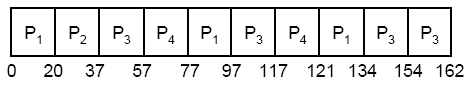
·         Average Waiting Time

= (P1 + P2 + P3 + P4) / 4

=  [{0 + (77 – 20) + (121 – 97)} + 20 + {37 + (97-57) + (134 – 117)} + {57 + (117 – 77)}] / 4

=  (81+20+94+97) / 4                     = 73 milliseconds

If there are n processes in the ready queue and the time quantum is q, then each process gets 1/n of the CPU time in chunks of at most q time units. Each process must wait no longer than (n – 1 ) x q time units until its next time quantum. For example, there are 5 processes and a time quantum of 20 milliseconds, each process will get up to 20 milliseconds every 100 milliseconds.

The performance of the RR algorithm depends heavily on the size of the time quantum.

·         If the time quantum is extremely large, the RR policy is similar to FCFS policy.

·         If the time quantum is extremely small (say 1 millisecond), the RR approach is called processor sharing and creates the appearance that each of n processes has its own processor running at 1/n speed of the real processor.

Fig: Quantum time and context switching

Turnaround time varies with the time quantum

Fig: Quantum time and Turnaround Time

Highest-Response Ration Next (HRN) Scheduling

Highest Response Ratio Next (HRRN) scheduling is a non-preemptive discipline, in which the priority of each job is dependent on its estimated run time, and also the amount of time it has spent waiting. Jobs gain higher priority the longer they wait, which prevents indefinite postponement (process starvation).

It selects a process with the largest ratio of waiting time over service time. This guarantees that a process does not starve due to its requirements.

In fact, the jobs that have spent a long time waiting compete against those estimated to have short run times.

Priority = waiting time + estimated runtime / estimated runtime

(Or)

Ratio = (waiting time + service time) / service time

Advantages

·         Improves upon SPF scheduling

·         Still non-preemptive

·         Considers how long process has been waiting

·         Prevents indefinite postponement

Disadvantages

·         Does not support external priority system. Processes are scheduled by using internal priority system.

Example: Consider the Processes with following Arrival time, Burst Time and priorities

Process	Arrival time	Burst time	Priority
P1	0	7	3 (High)
P2	2	4	1 (Low)
P3	3	4	2

Solution: HRRN

At time 0 only process p1 is available, so p1 is considered for execution

Since it is Non-preemptive, it executes process p1 completely. It takes 7 ms to complete process p1 execution.

Now, among p2 and p3 the process with highest response ratio is chosen for execution.

Ratio for p2    =          (5 + 4) / 4      =      2.25

Ratio for p3    =          (4 + 4) / 4      =      2

As process p2 is having highest response ratio than that of p3. Process p2 will be considered for execution and then followed by p3.

Average waiting time    = 0 + (7 - 2) + (11 - 3) / 3 =      4.33

Average Turnaround time =                              7 + (11 - 2) + (15 - 3) / 3        =                                 9.33

Interprocess Communication and synchronization

Introduction

Inter-process communication (IPC) is a set of techniques for the exchange of data among multiple threads in one or more processes.  This allows a program to handle many user requests at the same time. IPC facilitates efficient message transfer between processes.

IPC allows one application to control another application, thereby enabling data sharing without interference.

Race condition

A race condition occurs when two processes (or threads) access the same variable/resource without doing any synchronization that means when several processes access and manipulate the same data concurrently and the outcome of the execution depends on the particular order in which access takes place is called a race condition.

·         One process is doing a coordinated update of several variables

·         The second process observing one or more of those variables will see inconsistent results

·         Final outcome dependent on the precise timing of two processes

Example

·         One process is changing the balance in a bank account while another is simultaneously observing the account balance and the last activity date

·         Now, consider the scenario where the process changing the balance gets interrupted after updating the last activity date but before updating the balance

·         If the other process reads the data at this point, it does not get accurate information (either in the current or past time)

Critical Regions

Suppose two or more processes require access to a single non-sharable resource such as a printer. During the course of execution, each process will sending commands to the I/O device, receives status information, sending data, and / or receiving data. Such resource is called critical resource and the portion of the program that uses it is called critical section of the program. However only one program at a time be allowed in its critical section.

When two or more processes access shared data, often the data must be protected during access. Typically, a process that reads data from a shared queue cannot read it at the same time as the data is currently being written or its value being changed. Where a process is considered that it cannot be interrupted at the same time as performing a critical function such as updating data, it is prevented from being interrupted by the operating system till it has completed the update. During this time, the process is said to be in its critical section that means the part of the program where the shared memory is accessed is called critical section or critical region. Once the process has written the data, it can then be interrupted and other processes can also run.

Problems occur only when both tasks attempt to read and write the data at the same time. The answer is simple, lock the data structure whilst accessing (semaphores or interrupts disabled). There is no need for data locking if both processes only read at same time. Critical sections of a process should be small so that they do not take long to execute and thus other processes can run.

Semaphore

Semaphores are a technique for coordinating or synchronizing activities in which multiple processes compete for the same operating system resources.

Semaphores are commonly used for two purposes: to share a common memory space and to share access to files.

A semaphore is a value in a designated place in operating system (or kernel) storage that each process can check and then change. Depending on the value that is found, the process can use the resource or will find that it is already in use and must wait for some period before trying again. Semaphores can be binary (0 or 1) or can have additional values. Typically, a process using semaphores checks the value and then, if it using the resource, changes the value to reflect this so that subsequent semaphore users will know to wait.